फाईल:Airflow-Obstructed-Duct.png
नेविगेशन प जा
खोज प जा
इ पूर्वावलोकन के आकार: ८०० × ५७१ पिक्सेल । आरू दोसरो रेसोल्यूशन्स:३२० × २२९ पिक्सेल | ६४० × ४५७ पिक्सेल | १,०२४ × ७३१ पिक्सेल | १,२७० × ९०७ पिक्सेल.
संपूर्ण रिजोल्यूशन (१,२७० × ९०७ चित्रतत्व, संचिका के आकार: ८५ KB, MIME प्रकार: image/png)
सारांश

|
File:N S Laminar.svg इस फ़ाइल का एक वेक्टर संस्करण है।. जब अवर न हो, इस PNG फ़ाइल की जगह इसका उपयोग किया जाना चाहिए।
File:Airflow-Obstructed-Duct.png → File:N S Laminar.svg
अधिक जानकारी के लिए Help:SVG देखें। |
 |
| विवरण |
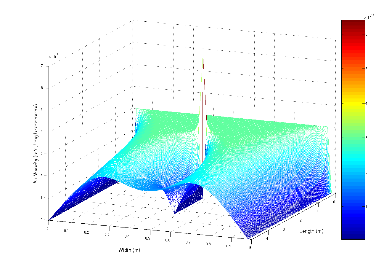
A simulation using the navier-stokes differential equations of the aiflow into a duct at 0.003 m/s (laminar flow). The duct has a small obstruction in the centre that is parallel with the duct walls. The observed spike is mainly due to numerical limitations. This script, which i originally wrote for scilab, but ported to matlab (porting is really really easy, mainly convert comments % -> // and change the fprintf and input statements) Matlab was used to generate the image.
%Matlab script to solve a laminar flow
%in a duct problem

%Constants
inVel = 0.003; % Inlet Velocity (m/s)
fluidVisc = 1e-5; % Fluid's Viscoisity (Pa.s)
fluidDen = 1.3; %Fluid's Density (kg/m^3)

MAX_RESID = 1e-5; %uhh. residual units, yeah...
deltaTime = 1.5; %seconds?
%Kinematic Viscosity
fluidKinVisc = fluidVisc/fluidDen;

%Problem dimensions
ductLen=5; %m
ductWidth=1; %m

%grid resolution
gridPerLen = 50; % m^(-1)
gridDelta = 1/gridPerLen;
XVec = 0:gridDelta:ductLen-gridDelta;
YVec = 0:gridDelta:ductWidth-gridDelta;

%Solution grid counts
gridXSize = ductLen*gridPerLen;
gridYSize = ductWidth*gridPerLen;

%Lay grid out with Y increasing down rows
%x decreasing down cols
%so subscripting becomes (y,x) (sorry)
velX= zeros(gridYSize,gridXSize);
velY= zeros(gridYSize,gridXSize);
newVelX= zeros(gridYSize,gridXSize);
newVelY= zeros(gridYSize,gridXSize);

%Set initial condition

for i =2:gridXSize-1
for j =2:gridYSize-1
velY(j,i)=0;
velX(j,i)=inVel;
end
end

%Set boundary condition on inlet
for i=2:gridYSize-1
velX(i,1)=inVel;
end

disp(velY(2:gridYSize-1,1));

%Arbitrarily set residual to prevent
%early loop termination
resid=1+MAX_RESID;

simTime=0;

while(deltaTime)
 count=0;
while(resid > MAX_RESID && count < 1e2)
 count = count +1;
for i=2:gridXSize-1
for j=2:gridYSize-1
newVelX(j,i) = velX(j,i) + deltaTime*( fluidKinVisc / (gridDelta.^2) * ...
(velX(j,i+1) + velX(j+1,i) - 4*velX(j,i) + velX(j-1,i) + ...
velX(j,i-1)) - 1/(2*gridDelta) *( velX(j,i) *(velX(j,i+1) - ...
velX(j,i-1)) + velY(j,i)*( velX(j+1,i) - velX(j,i+1))));

newVelY(j,i) = velY(j,i) + deltaTime*( fluidKinVisc / (gridDelta.^2) * ...
(velY(j,i+1) + velY(j+1,i) - 4*velY(j,i) + velY(j-1,i) + ...
velY(j,i-1)) - 1/(2*gridDelta) *( velY(j,i) *(velY(j,i+1) - ...
velY(j,i-1)) + velY(j,i)*( velY(j+1,i) - velY(j,i+1))));
end
end

%Copy the data into the front
for i=2:gridXSize - 1
for j = 2:gridYSize-1
velX(j,i) = newVelX(j,i);
velY(j,i) = newVelY(j,i);
end
end

%Set free boundary condition on inlet (dv_x/dx) = dv_y/dx = 0
for i=1:gridYSize
velX(i,gridXSize)=velX(i,gridXSize-1);
velY(i,gridXSize)=velY(i,gridXSize-1);

    end

    %y velocity generating vent
    for i=floor(2/6*gridXSize):floor(4/6*gridXSize)
        velX(floor(gridYSize/2),i) = 0;
        velY(floor(gridYSize/2),i-1) = 0;
    end

%calculate residual for
%conservation of mass
resid=0;
for i=2:gridXSize-1
for j=2:gridYSize-1
%mass continuity equation using central difference
%approx to differential
resid = resid + (velX(j,i+ 1)+velY(j+1,i) - ...
(velX(j,i-1) + velX(j-1,i)))^2;
end
end

resid = resid/(4*(gridDelta.^2))*1/(gridXSize*gridYSize);
fprintf('Time %5.3f \t log10Resid : %5.3f\n',simTime,log10(resid));


simTime = simTime + deltaTime;
end
mesh(XVec,YVec,velX)
deltaTime = input('\nnew delta time:');
end
%Plot the results
mesh(XVec,YVec,velX)
|
| तिथि | २४ फरवरी २००७ (original upload date) |
| स्रोत | Transferred from en.wikipedia to Commons. |
| लेखक | अंग्रेज़ी विकिपीडिया पर User A1 |
लाइसेन्सिंग
| इस कार्य को इसके लेखक, अंग्रेज़ी विकिपीडिया पर User A1 द्वारा सार्वजनिक डोमेन में प्रकाशित किया गया है। यह पूरे विश्व में लागू होता है। कुछ देशों में यह कानूनी तौर पर नहीं हो सकता है; ऐसा हो तो: User A1 सभी को इस कार्य का इस्तेमाल किसी भी उद्देश्य से, बिना किसी बाधाओं के इन शर्तों के कानून द्वारा अनिवार्य किए तक करने की अनुमति देता/देती हैं। |
मूल अपलोड लॉग
The original description page was here. All following user names refer to en.wikipedia.
- 2007-02-24 05:45 User A1 1270×907×8 (86796 bytes) A simulation using the navier-stokes differential equations of the aiflow into a duct at 0.003 m/s (laminar flow). The duct has a small obstruction in the centre that is paralell with the duct walls. The observed spike is mainly due to numerical limitatio
फाइल केरौ इतिहास
संचिका पुरानौ समय मँ कैन्हौ दिखै छेलै इ जानै लेली वांछित दिनांक/समय प चाँपौ।
| दिनांक/समय | थंबनेल | आयाम | सदस्य | टिप्पणी | |
|---|---|---|---|---|---|
| वर्तमान | १६:५२, १ मई २००७ | | १,२७० × ९०७ (८५ KB) | wikimediacommons>Smeira | {{Information |Description=A simulation using the navier-stokes differential equations of the aiflow into a duct at 0.003 m/s (laminar flow). The duct has a small obstruction in the centre that is paralell with the duct walls. The observed spike is mainly |
फाइल केरौ उपयोग
ई फ़ाइल के प्रयोग नीच्चाँ देलौ गेलौ पन्ना प होय रहलौ छै: